In order to digest the multitude of data transmitted from robots at each of our customer sites, engineering teams at 6 River Systems developed a data pipeline to ship data from the robotic operating system (ROS) to Google BigQuery. What does this infrastructure look like and how did we develop it? This blog post will provide an overview of the design and then discuss our open sourced implementation.
First, why did we need to develop this pipeline?
Aren’t there existing technologies for shipping data to a cloud server? Let’s talk about some of our goals for this project.
We needed a system that:
- Can collect information from all of our robots at all of our sites and store it in one location.
While there is value in looking at the information from a single robot or single site, we also look for trends across our entire fleet. Using this pathway, we can compare different robots on different software versions at different sites. - Can operate with limited network connectivity.
Our AMRs, which we call Chucks, do not require any additional infrastructure at our customer sites. This allows us to deploy in a fraction of the time of other solutions. However, it comes with some constraints, one of which is that we do not always have perfect network connectivity across the entirety of every warehouse. Our solution needs to be able to buffer data if there is a gap in network coverage. - Does not lose any data.
Analysis is limited by the quality and completeness of the data available. Regardless of what happens to a robot, whether it powers down or loses connectivity, we want to make sure that information from it makes it to the cloud. - Is easy to expand / add information to in the future.
We are in the business of continuous improvement. As we create new features, we must constantly expand the scope of analytics information that we are collecting. It should be simple for any developer to add additional data. - Leverages technologies that we are already using in other parts of our stack.
There is no need to reinvent the wheel if we already have experience with technology.
Given those goals, we developed the following pipeline:
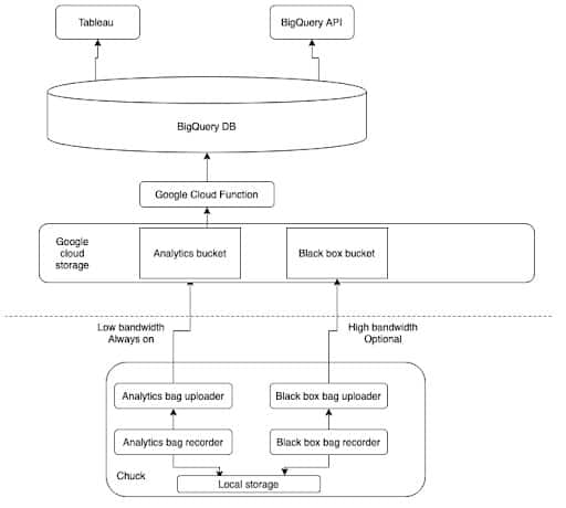
Let’s talk through this block diagram piece by piece.
Local Storage
First, on the bottom of the stack we have processes running on each individual robot. Chucks run using a collection of tools and libraries called ROS (Robot Operating System). ROS is used across a wide array of robotic tech stacks, both in academia and industry. ROS provides a lot of tools. Important to this discussion, ROS has an interprocess communication system called ROS topics which send messages between different nodes. These messages can be recorded to disk in a file called a bag or rosbag. Rosbags are useful because they can be played back offline to view data using the ROS visualization tools.
Chucks are continuously recording two types of rosbags: black box and analytics. The black box bags are like the data recorder on an airplane. They contain high bandwidth sensor data to allow us to recreate what a robot was seeing and doing. These bags are stored on disk and optionally uploaded to the cloud. Analytics bags are used for our data pipeline. Any ROS topic can be included into our analytics bags, though we want to keep the bag size in check so that it does not impact customer network bandwidth. As such, these bags do not contain things such as raw sensor data. A new analytics bag is saved every 2 minutes and then uploaded to the cloud.
Google Cloud Storage
Now we move up the diagram to the cloud portion of the stack. We leverage a number of different technologies that are part of the Google Cloud offerings. Google provides a suite of tools that makes it easy to use their various cloud services.
For our Chuck analytics pipeline, we use a combination of three of their products. First, we use Google Cloud Storage (GCS) as the staging point for our data. The bags are uploaded into a GCS bucket. The storage bucket allows us to keep our data in bag form for easy download to use with other ROS tools. It also provides a number of guarantees around uptime and durability so we know that none of our data will get lost. On the robot, we use Google’s storage SDK and custom code to ensure that each bag gets uploaded into the storage bucket. Our system deletes bags from the robot once they have made it to the cloud and periodically checks to see if any old bags still need to be uploaded. In this way, we can ensure that all of our analytics data makes it into the cloud even if the robot is traveling through an area of poor network connectivity.
Once a bag is uploaded, it triggers the invocation of a Google Cloud Function (GCF). A GCF is a serverless process running in the cloud. It’s a single function that gets called on for each bag. Google provides automatic scaling, so no matter how many robots are running, we always have just enough GCF instances running to handle all the bags being uploaded without any being idle. Our GCF opens the bag up, converts the data, and inserts it into its final storage place in our pipeline.
The Data Warehouse and Analysis
The final two levels of our diagram is 6RS-side. The data from the bag is inserted into a BigQuery. BigQuery is a data warehouse product from Google designed specifically for analytics applications. Data is stored in tables and can be accessed using standard SQL queries or with a variety of different products that integrate with it. At 6RS, we use direct SQL queries for quick analysis, Tableau for data visualization, and Google Colab for data analysis. For example, we store robot velocity data at a regular cadence. This allows us to answer all kinds of questions: what is the average speed across the entire fleet? Are there some individual robots that are unreasonably slow? At a single customer site, are there some aisles which are much slower than others? These insights can be used to monitor our fleet and proactively help our customers. Here is an anonymized example of average robot speed per aisle:
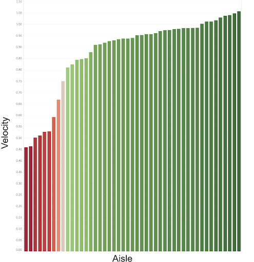
As you can see, most aisles have a similar average speed, but there are a few aisles where the average speed is significantly lower. Note that this chart does not include intra-aisle speed, which is typically significantly faster. We can use this information to help the site management understand why Chucks are slower in those aisles and take steps to mitigate the problem.
But, in this blog post, we are focusing on the pipeline, not the outputs. Check back next month for the next post in this series in which we will discuss in more detail how we can extract useful insights from the data collected in this pipeline.
Now, for the engineers who want a bit more technical insight, let’s look at some of the design decisions that we made when developing this pipeline.
Typescript
First, we chose to write our function in Typescript. We chose this for a few reasons.
At 6RS, most of our code is developed in either Typescript or C++ so we wanted to stick with something familiar to most engineers at the company.
Google provides a nodejs runtime for their cloud functions and a nodejs BigQuery API.
Cruise automation had developed a rosbag parsing library in javascript that we could leverage. Our forked version can be found here.
Serverless
Next, we chose serverless as the framework for deployment. Serverless provides an easy to use framework to deploy into different cloud function infrastructures, including Google, AWS, etc. This project was our first experiment using serverless at 6RS, and we liked how it made the deployment process simpler.
Cloud function
Finally, we had to make a number of design decisions for how we mapped our rosbags of data into BigQuery tables. Our main focus was on having the GCF be essentially “set it and forget it:” we did not want to have to update our parsing function every time we wanted to add new information to our datasets.
We also focused on ease of use for developers. It should be simple to add more data to the dataset and easy to know what it will look like once it is in the database. To do this, we designed our pipeline such that every topic in the bag maps to a table in BigQuery with the same name. If a new topic is added to the bag, the GCF automatically makes a new table. The schema for the table is generated from the structure of the message such that every field in the message becomes a column in the table. Each individual message is a separate row. If we update the message to include new fields in the future, the schema is automatically updated to be the union of the two messages. That way, the function can operate on any version of the data as the new version is rolled across our fleet of robots.
To make data analysis easier, we append common information to every row of the table, including the robot’s pose, the timestamp at which the message was recorded, the robot ID, and the build number. This way, this data does not need to be included in every single ROS message being stored in the analytics bag.
Our google cloud function is available at github.com/6RiverSystems/RosbagToBigQuery. I encourage you to open the repository (at tag v1.0) to see how the following design decisions play out in actual code.
The code in this repository is a slimmed down version of our GCF, but it should be deployable and work to move data from bags into BigQuery. If you encounter any problems, please open an issue or a PR in the repository.
Check back later for the next blog post in this series where we discuss how we can query this data and use insights from it to drive our product decisions.
We’re building a wicked awesome team.
Check our current job postings to see if there’s a role for you.
About the Author

Dan has worked on robotic movement for his whole career. He helped develop a variety of robotic platforms, including an autonomous off road vehicle, a hospital delivery robot, an autonomous tugger for distribution warehouses, a number of different micro aerial vehicles, and now Chuck.
Dan has a B.S.E. from Olin College of Engineering and an M.Sc. in Robotics, Systems and Controls from ETH Zürich.

